Table of Contents
Introduction
In this section, we describe solvers of ordinary differential equations (ODE) characterized by the following equation:
\[ \frac{\mathrm{d} \vec u(t)}{\mathrm{d}t} = \vec f( t, \vec u(t)) \text{ on } (0,T), \]
and the initial condition
\[ \vec u( 0 ) = \vec u_{ini}, \]
where \( T>0 \). This class of problems can be solved by TNL::Solvers::ODE::ODESolver which incorporates the following template parameters:
- Method - specifies the numerical method used for solving the ODE.
- Vector - denotes a container used to represent the vector \( \vec u(t) \).
- SolverMonitor - is a tool for tracking the progress of the ODE solver.
Method
TNL provides several methods for ODE solution, categorized based on their order of accuracy:
1-st order accuracy methods:
- TNL::Solvers::ODE::Methods::Euler or TNL::Solvers::ODE::Methods::Matlab::ode1 - the forward Euler method.
- TNL::Solvers::ODE::Methods::Midpoint - the explicit midpoint method.
2-nd order accuracy methods:
- TNL::Solvers::ODE::Methods::Heun2 or TNL::Solvers::ODE::Methods::Matlab::ode2 - the Heun method with adaptive choice of the time step.
- TNL::Solvers::ODE::Methods::Ralston2 - the Ralston method.
- TNL::Solvers::ODE::Methods::Fehlberg2 - the Fehlberg method with adaptive choice of the time step.
3-rd order accuracy methods:
- TNL::Solvers::ODE::Methods::Kutta - the Kutta method.
- TNL::Solvers::ODE::Methods::Heun3 - the Heun method.
- TNL::Solvers::ODE::Methods::VanDerHouwenWray - the Van der Houwen/Wray method.
- TNL::Solvers::ODE::Methods::Ralston3 - the Ralston method.
- TNL::Solvers::ODE::Methods::SSPRK3 - the Strong Stability Preserving Runge-Kutta method.
- TNL::Solvers::ODE::Methods::BogackiShampin or TNL::Solvers::ODE::Methods::Matlab::ode23 - Bogacki-Shampin method with adaptive choice of the time step.
4-th order accuracy methods:
- TNL::Solvers::ODE::Methods::OriginalRungeKutta - the "original" Runge-Kutta method.
- TNL::Solvers::ODE::Methods::Rule38 - 3/8 rule method.
- TNL::Solvers::ODE::Methods::Ralston4 - the Ralston method.
- TNL::Solvers::ODE::Methods::KuttaMerson - the Runge-Kutta-Merson method with adaptive choice of the time step.
5-th order accuracy methods:
- TNL::Solvers::ODE::Methods::CashKarp - the Cash-Karp method with adaptive choice of the time step.
- TNL::Solvers::ODE::Methods::DormandPrince or TNL::Solvers::ODE::Methods::Matlab::ode45 - the Dormand-Prince with adaptive choice of the time step.
- TNL::Solvers::ODE::Methods::Fehlberg5 - the Fehlberg method with adaptive choice of the time step.
Vector
The vector \( \vec u(t) \) in ODE solvers can be represented using different types of containers, depending on the size and nature of the ODE system:
- Static vectors (TNL::Containers::StaticVector): This is suitable for small systems of ODEs with a fixed number of unknowns. Utilizing StaticVector allows the ODE solver to be executed within GPU kernels. This capability is particularly useful for scenarios like running multiple sequential solvers in parallel, as in the case of TNL::Algorithms::parallelFor.
- Dynamic vectors (TNL::Containers::Vector or TNL::Containers::VectorView): These are preferred when dealing with large systems of ODEs, such as those arising in the solution of parabolic partial differential equations using the method of lines. In these instances, the solver typically handles a single, large-scale problem that can be executed in parallel internally.
Static ODE solvers
Scalar problem
Static solvers are primarily intended for scenarios where \( x \in R \) is scalar or \( \vec x \in R^n \) is vector with a relatively small dimension. We will demonstrate this through a scalar problem defined as follows:
\[ \frac{\mathrm{d}u}{\mathrm{d}t} = t \sin ( t ) \text{ on } (0,T), \]
with the initial condition
\[ u( 0 ) = 0. \]
First, we define the Real type to represent floating-point arithmetic, here chosen as double.
Next we define the main function of the solver:
We begin the main function by defining necessary types:
We set Vector as StaticVector with a size of one. We also choose the basic Euler method as the Method. Finally, we construct the ODESolver type.
Next we define the time-related variables:
Here:
- final_t represents the size of the time interval \( (0,T)\).
- tau is the integration time step.
- output_time_step denotes checkpoints in which we will print value of the solution \( u(t)\).
Next, we initialize the solver:
We create an instance of the ODESolver, set the integration time step (using setTau) and the initial time of the solver with setTime. Then, we initialize the variable u (representing the ODE solution) to the initial state \( u(0) = 0\).
We proceed to the main loop iterating over the time interval \( (0,T) \):
We iterate with the time variable \( t \) (represented by getTime) until the time \( T \) (represented by final_t) with step given by the frequency of the checkpoints (represented by output_time_steps). We let the solver to iterate until the next checkpoint or the end of the interval \((0,T) \) depending on what occurs first (it is expressed by TNL::min(solver.getTime()+output_time_step,final_t)). The lambda function f represents the right-hand side \( f \) of the ODE being solved. The lambda function receives the following arguments:
- t is the current value of the time variable \( t \in (0,T)\),
- tau is the current integration time step,
- u is the current value of the solution \( u(t)\),
- fu is a reference on a variable into which we evaluate the right-hand side \( f(u,t) \) on the ODE.
The lambda function is supposed to compute just the value of fu. It is fu=t*sin(t) in our case. Finally we call the ODE solver (solver.solve(u,f)). As parameters, we pass the variable u representing the solution \( u(t)\) and a lambda function representing the right-hand side of the ODE. At the end, we print values of the solution at given checkpoints.
The complete example looks as:
The output is as follows:
These results can be visualized using several methods. One option is to use Gnuplot. The Gnuplot command to plot the data is:
Alternatively, the data can be processed and visualized using the following Python script, which employs Matplotlib for graphing.
The graph depicting the solution of the scalar ODE problem is illustrated below:

Lorenz system
In this example, we demonstrate the application of the static ODE solver in solving a system of ODEs, specifically the Lorenz system. The Lorenz system is a set of three coupled, nonlinear differential equations defined as follows:
\[ \frac{\mathrm{d}x}{\mathrm{d}t} = \sigma( x - y), \text{ on } (0,T), \]
\[ \frac{\mathrm{d}y}{\mathrm{d}t} = x(\rho - z ) - y, \text{ on } (0,T), \]
\[ \frac{\mathrm{d}z}{\mathrm{d}t} = xy - \beta z, \text{ on } (0,T), \]
with the initial condition
\[ \vec u(0) = (x(0),y(0),z(0)) = \vec u_{ini}. \]
Here, \( \sigma, \rho \) and \( \beta \) are given constants. The solution of the system, \( \vec u(t) = (x(t), y(t), z(t)) \in R^3 \) is represented by three-dimensional static vector (TNL::Containers::StaticVector).
The implementation of the solver for the Lorenz system is outlined below:
This code shares similarities with the previous example, with the following key differences:
- We define the type Vector of the variable u representing the solution \( \vec u(t) \) as TNL::Containers::StaticVector< 3, Real >, i.e. static vector with size of three.
- Alongside the solver parameters (final_t, tau and output_time_step) we define the Lorenz system's parameters (sigma, rho and beta). 27 const Real sigma = 10.0;28 const Real rho = 28.0;29 const Real beta = 8.0 / 3.0;
- The initial condition is \( \vec u(0) = (1,2,3) \). 39 Vector u( 1.0, 2.0, 3.0 );
- In the lambda function, which represents the right-hand side of the Lorenz system, auxiliary aliases x, y, and z are defined for readability. The main computation for the right-hand side of the system is implemented subsequently. 46 auto f = [ = ]( const Real& t, const Real& tau, const Vector& u, Vector& fu )47 {48 const Real& x = u[ 0 ];49 const Real& y = u[ 1 ];50 const Real& z = u[ 2 ];51 fu[ 0 ] = sigma * ( y - x );52 fu[ 1 ] = rho * x - y - x * z;53 fu[ 2 ] = -beta * z + x * y;54 };
- In the remaining part of the time loop, we simply execute the solver, allowing it to evolve the solution until the next snapshot time. At this point, we also print the current state of the solution to the terminal.
The solver generates a file containing the solution values \( (\sigma(i \tau), \rho( i \tau), \beta( i \tau )) \) for each time step, where \( i = 0, 1, \ldots N \). These values are recorded on separate lines. The content of the output file is structured as follows:
The output file generated by the solver can be visualized in various ways. One effective method is to use Gnuplot, which allows for interactive 3D visualization. The Gnuplot command for plotting the data in 3D is:
Alternatively, the data can also be processed using the following Python script:
This script is structured similarly to the one in the previous example. It processes the output data and creates a visual representation of the solution.
The resultant visualization of the Lorenz problem is shown below:

Combining static ODE solvers with parallel for
Static solvers can be effectively utilized within lambda functions in conjunction with TNL::Algorithms::parallelFor. This approach is particularly beneficial when there's a need to solve a large number of independent ODE problems, such as in parametric analysis scenarios. We will demonstrate this application using the two examples previously described.
Solving scalar problems in parallel
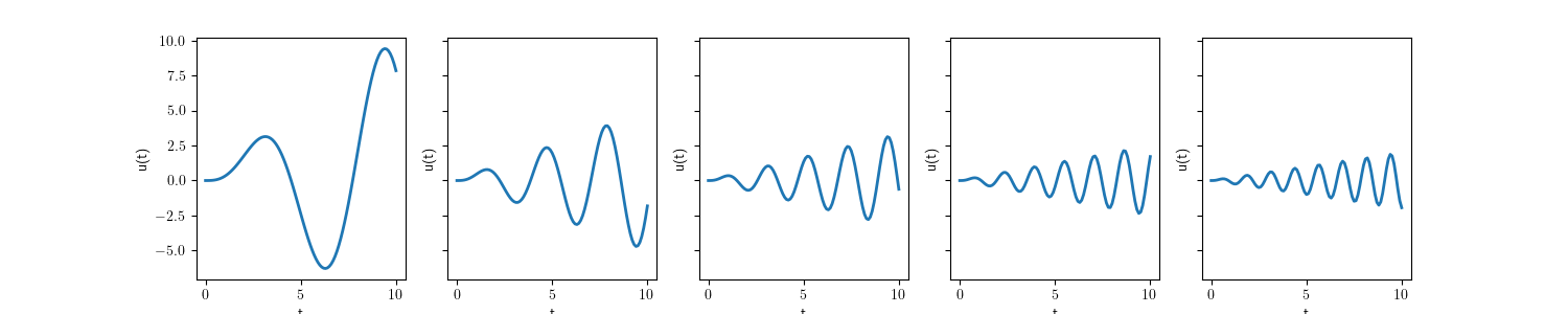
The first example addresses an ODE defined by the following equation
\[ \frac{\mathrm{d}u}{\mathrm{d}t} = t \sin ( c t ) \text{ on } (0,T), \]
and the initial condition
\[ u( 0 ) = 0, \]
where \( c \) is a constant. We aim to solve this ODE in parallel for a range of values \( c \in \langle c_{min}, c_{max} \rangle \). The exact solution for this equation is available here. The implementation for this parallel computation is detailed in the following code:
In this example, we demonstrate how to execute the ODE solver on a GPU. To facilitate this, the main solver logic has been encapsulated within a separate function, solveParallelODEs, which accepts a template parameter Device indicating the target device for execution. The results from individual ODE solutions are stored in memory and eventually written to a file named file_name. The variable \( u \), being scalar, is represented by the type TNL::Containers::StaticVector<1,Real> within the solver.
Next, we define the parameters of the ODE solver (final_t, tau and output_time_step) as shown:
The interval for the ODE parameter \( c \in \langle c_{min}, c_{max} \rangle \) ( c_min, c_max, ) is established, along with the number of values c_vals distributed equidistantly in the interval, determined by the step size c_step.
We use the range of different c values as the range for the parallelFor loop. This loop processes the lambda function solve. Before diving into the main lambda function, we allocate the vector results for storing the ODE problem results at different time levels. As data cannot be directly written from GPU to an output file, results serves as intermediary storage. Additionally, to enable GPU access, we prepare the vector view results_view.
Proceeding to the main lambda function solve:
This function receives idx, the index of the value of the parameter c. After calculating c, we create the ODE solver solver and set its parameters using setTau and setTime. We also set the initial condition of the ODE and define the variable time_step to count checkpoints, which are stored in memory using results_view.
In the time loop, we iterate over the interval \( (0, T) \), setting the solver’s stop time with setStopTime and running the solver with solve.
Each checkpoint's result is then stored in the results_view.
It's important to note how the parameter c is passed to the lambda function f. The solve method of ODE solvers accepts user-defined parameters through variadic templates. This means additional parameters like c can be included alongside u and the right-hand side f, and are accessible within the lambda function f.
Due to limitations of the nvcc compiler, which does not accept lambda functions defined within another lambda function, the f lambda function cannot be defined inside the solve lambda function. Therefore, c, defined in solve, cannot be captured by f.
The solver outputs a file in the following format:
The file can be visuallized using Gnuplot as follows
or it can be processed by the following Python script:
The result of this example looks as follows:
Solving the Lorenz system in parallel
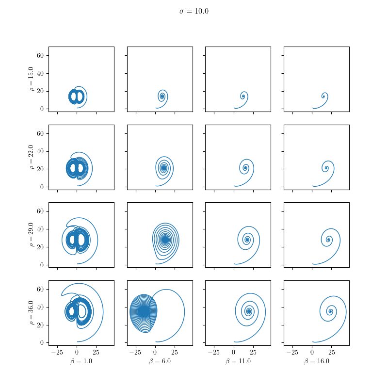
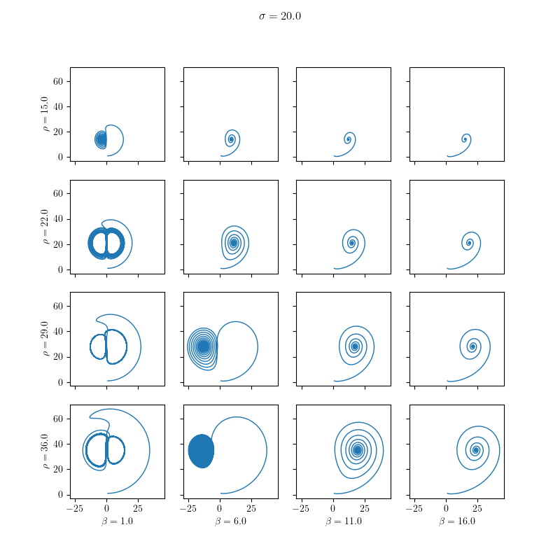
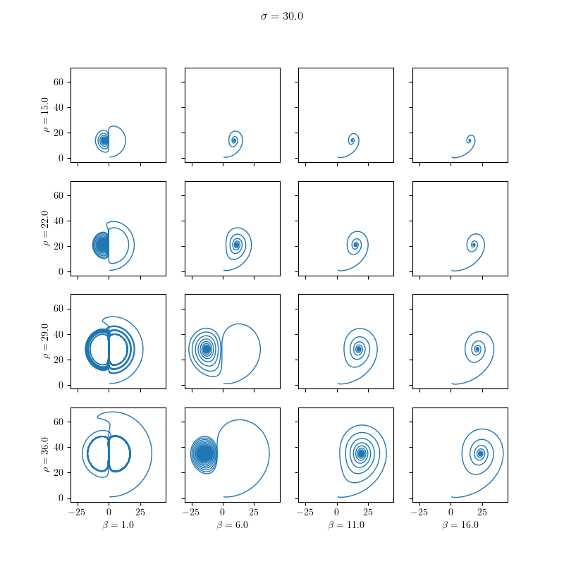
The second example is a parametric analysis of the Lorenz model
\[ \frac{\mathrm{d}x}{\mathrm{d}t} = \sigma( x - y), \text{ on } (0,T) \]
\[ \frac{\mathrm{d}y}{\mathrm{d}t} = x(\rho - z ) - y, \text{ on } (0,T) \]
\[ \frac{\mathrm{d}z}{\mathrm{d}t} = xy - \beta z, \text{ on } (0,T) \]
with the initial condition
\[ \vec u(0) = (x(0),y(0),z(0)) = \vec u_{ini}. \]
We solve it for different values of the model parameters:
\[ \sigma_i = \sigma_{min} + i \Delta \sigma, \]
\[ \rho_j = \rho_{min} + j \Delta \rho, \]
\[ \beta_k = \beta_{min} + k \Delta \beta, \]
where we set \(( \Delta \sigma = \Delta \rho = \Delta \beta = l / (p-1) \)) and \(( i,j,k = 0, 1, \ldots, p - 1 \)). The code of the solver looks as follows:
It is very similar to the previous one. There are just the following changes:
Since we are analysing dependence on three parameters, we involve a three-dimensional parallelFor. For this, we introduce a type for a three-dimensional multiindex.
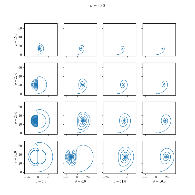
11using Real = double;We define minimal values for the parameters \( \sigma \in [10,40], \beta \in [15, 36] \) and \( \rho \in [1,16]\) and set the number of different values for each parameter by parametric_steps. The size of equidistant steps (sigma_steps, rho_steps and beta_steps) in the parameter variations is also set.
31 const Real sigma_min = 10.0;32 const Real rho_min = 15.0;33 const Real beta_min = 1.0;34 const int parametric_steps = 4;35 const Real sigma_step = 30.0 / ( parametric_steps - 1 );36 const Real rho_step = 21.0 / ( parametric_steps - 1 );37 const Real beta_step = 15.0 / ( parametric_steps - 1 );Next, we allocate vector results for storing the solution of the Lorenz problem for various parameters.
42 const int results_size( output_time_steps * parametric_steps * parametric_steps * parametric_steps );43 TNL::Containers::Vector< StaticVector, Device > results( results_size, 0.0 );44 auto results_view = results.getView();We define the lambda function f for the right-hand side of the Lorenz problem and the lambda function solve for the ODE solver, with a specific setup of the parameters.
49 const Real& t,50 const Real& tau,51 const StaticVector& u,52 StaticVector& fu,53 const Real& sigma_i,54 const Real& rho_j,55 const Real& beta_k )56 {57 const Real& x = u[ 0 ];58 const Real& y = u[ 1 ];59 const Real& z = u[ 2 ];60 fu[ 0 ] = sigma_i * ( y - x );61 fu[ 1 ] = rho_j * x - y - x * z;62 fu[ 2 ] = -beta_k * z + x * y;63 };and the lambda function solve representing the ODE solver for the Lorenz problem
68 {70 const Real sigma_i = sigma_min + idx[ 0 ] * sigma_step;71 const Real rho_j = rho_min + idx[ 1 ] * rho_step;72 const Real beta_k = beta_min + idx[ 2 ] * beta_step;7476 ODESolver solver;77 solver.setTau( tau );78 solver.setTime( 0.0 );79 StaticVector u( 1.0, 1.0, 1.0 );80 int time_step( 1 );81 results_view[ ( idx[ 0 ] * parametric_steps + idx[ 1 ] ) * parametric_steps + idx[ 2 ] ] = u;8385 while( time_step < output_time_steps ) {86 solver.setStopTime( TNL::min( solver.getTime() + output_time_step, final_t ) );88 solver.solve( u, f, sigma_i, rho_j, beta_k );90 const int k =91 ( ( time_step++ * parametric_steps + idx[ 0 ] ) * parametric_steps + idx[ 1 ] ) * parametric_steps + idx[ 2 ];92 results_view[ k ] = u;93 }95 };with setup of the parameters
76 ODESolver solver;77 solver.setTau( tau );78 solver.setTime( 0.0 );79 StaticVector u( 1.0, 1.0, 1.0 );80 int time_step( 1 );81 results_view[ ( idx[ 0 ] * parametric_steps + idx[ 1 ] ) * parametric_steps + idx[ 2 ] ] = u;The solve lambda function is executed using a three-dimensional parallelFor (TNL::Algorithms::parallelFor). We define multi-indexes begin and end for this purpose:
101 TNL::Algorithms::parallelFor< Device >( begin, end, solve );- The lambda function solve takes a multi-index idx, which is used to compute specific values for \( \sigma_i, \rho_j, \beta_k \), denoted as sigma_i, rho_j, and beta_k: These parameters must be explicitly passed to the lambda function f. This necessity arises due to the nvcc compiler's limitation of not accepting a lambda function defined within another lambda function, as mentioned before:70 const Real sigma_i = sigma_min + idx[ 0 ] * sigma_step;71 const Real rho_j = rho_min + idx[ 1 ] * rho_step;72 const Real beta_k = beta_min + idx[ 2 ] * beta_step;88 solver.solve( u, f, sigma_i, rho_j, beta_k );
The initial condition for the Lorenz problem is set to vector \( (1,1,1) \):
76 ODESolver solver;77 solver.setTau( tau );78 solver.setTime( 0.0 );79 StaticVector u( 1.0, 1.0, 1.0 );80 int time_step( 1 );81 results_view[ ( idx[ 0 ] * parametric_steps + idx[ 1 ] ) * parametric_steps + idx[ 2 ] ] = u;Subsequently, we initiate the time loop. Within this loop, we store the state of the solution in the vector view results_view at intervals defined by output_time_step:
85 while( time_step < output_time_steps ) {86 solver.setStopTime( TNL::min( solver.getTime() + output_time_step, final_t ) );88 solver.solve( u, f, sigma_i, rho_j, beta_k );90 const int k =91 ( ( time_step++ * parametric_steps + idx[ 0 ] ) * parametric_steps + idx[ 1 ] ) * parametric_steps + idx[ 2 ];92 results_view[ k ] = u;93 }Upon solving all ODEs, we transfer all solutions from the vector results to an output file:
105 std::fstream file;106 file.open( file_name, std::ios::out );107 for( int sigma_idx = 0; sigma_idx < parametric_steps; sigma_idx++ )108 for( int rho_idx = 0; rho_idx < parametric_steps; rho_idx++ )109 for( int beta_idx = 0; beta_idx < parametric_steps; beta_idx++ ) {110 Real sigma = sigma_min + sigma_idx * sigma_step;111 Real rho = rho_min + rho_idx * rho_step;112 Real beta = beta_min + beta_idx * beta_step;113 file << "# sigma " << sigma << " rho " << rho << " beta " << beta << '\n';114 for( int i = 0; i < output_time_steps - 1; i++ ) {115 int offset = ( ( i * parametric_steps + sigma_idx ) * parametric_steps + rho_idx ) * parametric_steps + beta_idx;116 auto u = results.getElement( offset );117 file << u[ 0 ] << " " << u[ 1 ] << " " << u[ 2 ] << '\n';118 }119 file << '\n';120 }
The output file has the following format:
It can be processed by the following Python script:
The results are visualized in the following images:
Dynamic ODE Solvers
In this section, we demonstrate how to solve the simple 1D heat equation, a parabolic partial differential equation expressed as:
\[\frac{\partial u(t,x)}{\partial t} - \frac{\partial^2 u(t,x)}{\partial^2 x} = 0 \text{ on } (0,T) \times (0,1), \]
with boundary conditions
\[u(t,0) = 0, \]
\[u(t,0) = 1, \]
and initial condition
\[u(0,x) = u_{ini}(x) \text{ on } [0,1]. \]
We discretize the equation by the finite difference method for numerical approximation. First, we define set of nodes \( x_i = ih \) for \(i=0,\ldots n-1 \) where \(h = 1 / (n-1) \) (adopting C++ indexing for consistency). Employing the method of lines and approximating the second derivative by the central finite difference
\[\frac{\partial^2 u(t,x)}{\partial^2 x} \approx \frac{u_{i-1} - 2 u_i + u_{i+1}}{h^2}, \]
we derive system of ODEs:
\[\frac{\mathrm{d} u_i(t)}{\mathrm{d}t} = \frac{u_{i-1} - 2 u_i + u_{i+1}}{h^2} \text{ for } i = 1, \ldots, n-2, \]
where \( u_i(t) = u(t,ih) \) represents the function value at node \( i \) and \( h \) is the spatial step between two adjacent nodes of the numerical mesh. The boundary conditions are set as:
\[u_0(t) = u_{n-1}(t) = 0 \text{ on } [0,T]. \]
What are the main differences compared to the Lorenz model?
- System Size and Vector Representation:
- The Lorenz model has a fixed size of three, representing the parameters \( (x, y, z) \) in \( R^3 \). This small, fixed-size vector can be efficiently represented using a static vector, specifically TNL::Containers::StaticVector< 3, Real >.
- In contrast, the size of the ODE system for the heat equation, as determined by the method of lines, varies based on the desired accuracy. The greater the value of \( n \), the more accurate the numerical approximation. The number of nodes \( n \) for spatial discretization defines the number of parameters or degrees of freedom, DOFs. Consequently, the system size can be large, necessitating the use of a dynamic vector, TNL::Containers::Vector, for solutions.
- Evaluation Approach and Parallelization:
- Due to its small size, the Lorenz model's right-hand side can be evaluated sequentially by a single thread.
- However, the ODE system for the heat equation can be very large, requiring parallel computation to efficiently evaluate its right-hand side.
- Data Allocation and Execution Environment:
- The dynamic vector TNL::Containers::Vector allocates data dynamically, which precludes its creation within a GPU kernel. As a result, ODE solvers cannot be instantiated within a GPU kernel.
- Therefore, the lambda function f, which evaluates the right-hand side of the ODE system, is executed on the host. It utilizes TNL::Algorithms::parallelFor to facilitate the parallel evaluation of the system's right-hand side.
Basic setup
The implementation of the solver for the heat equation is detailed in the following way:
The solver is encapsulated within the function solveHeatEquation, which includes a template parameter Device. This parameter specifies the device (e.g., CPU or GPU) on which the solver will execute. The implementation begins with defining necessary types:
- Vector is alias for TNL::Containers::Vector. The choice of a dynamic vector (rather than a static vector like TNL::Containers::StaticVector) is due to the potentially large number of degrees of freedom (DOFs) that need to be stored in a resizable and dynamically allocated vector.
- VectorView is designated for creating vector view, which is essential for accessing data within lambda functions, especially when these functions are executed on the GPU.
- Method defines the numerical method for time integration.
- ODESolver is the type of the ODE solver that will be used for calculating the time evolution in the time-dependent heat equation.
After defining these types, the next step in the implementation is to establish the parameters of the discretization:
- final_t represents the length of the time interval \( [0,T] \).
- output_time_step defines the time intervals at which the solution \( u \) will be written into a file.
- n stands for the number of DOFs, i.e. number of nodes used for the finite difference method.
- h is the space step, meaning the distance between two consecutive nodes.
- tau represents the time step used for integration by the ODE solver. For a second order parabolic problem like this, the time step should be proportional to \( h^2 \).
- h_sqr_inv is an auxiliary constant equal to \( 1/h^2 \). It is used later in the finite difference method for approximating the second derivative.
The initial condition \( u_{ini} \) is set as:
\[u_{ini}(x) = \left\{ \begin{array}{rl} 0 & \text{ for } x < 0.4, \\ 1 & \text{ for } 0.4 \leq x \leq 0.6, \\ 0 & \text{ for } x > 0. \\ \end{array} \right. \]
This initial condition defines the state of the system at the beginning of the simulation. It specifies a region (between 0.4 and 0.6) where the temperature (or the value of \( u \)) is set to 1, and outside this region, the temperature is 0.
After setting the initial condition, the next step is to write it to a file. This is done using the write function, which is detailed later.
Next, we create an instance of the ODE solver solver and set the integration time step tau of the solver (TNL::Solvers::ODE::ExplicitSolver::setTau ) The initial time is set to zero with (TNL::Solvers::ODE::ExplicitSolver::setTime).
Finally, we proceed to the time loop:
The time loop is executed, utilizing the time variable from the ODE solver (TNL::Solvers::ODE::ExplicitSolver::getTime). The loop iterates until reaching the end of the specified time interval \( [0, T] \), defined by the variable final_t. The stop time of the ODE solver is set with TNL::Solvers::ODE::ExplicitSolver::setStopTime, either to the next checkpoint for storing the state of the system or to the end of the time interval, depending on which comes first.
The lambda function f is defined to express the discretization of the second derivative of \( u \) using the central finite difference and to incorporate the boundary conditions.
The function receives the following parameters:
- i represents the index of the node, corresponding to the individual ODE derived from the method of lines. It is essential for evaluating the update of \( u_i^k \) to reach the next time level \( u_i^{k+1} \).
- u is a vector view representing the state \( u_i^k \) of the heat equation on the \( k-\)th time level.
- fu is a vector that stores updates or time derivatives in the method of lines which will transition \( u \) to the next time level.
In this implementation, the lambda function f plays a crucial role in applying the finite difference method to approximate the second derivative and in enforcing the boundary conditions, thereby driving the evolution of the system in time according to the heat equation.
In the lambda function f, the solution \( u \) remains unchanged on the boundary nodes. Therefore, the function returns zero for these boundary nodes. For the interior nodes, f evaluates the central difference to approximate the second derivative.
The lambda function time_stepping is responsible for computing updates for all nodes \( i = 0, \ldots, n-1 \). This computation is performed using TNL::Algorithms::parallelFor, which iterates over all the nodes and calls the function f for each one. Since the nvcc compiler does not support lambda functions defined within another lambda function, f is defined separately, and the parameters u and fu are explicitly passed to it.
The ODE solver is executed with solve. The current state of the heat equation u and the lambda function f (controlling the time evolution) are passed to the solve method. After each iteration, the current state is saved to a file using the write function.
The write function is used to write the solution of the heat equation to a file. The specifics of this function, including its parameters and functionality, are detailed in the following:
- file specifies the file into which the solution will be stored.
- u represents the solution of the heat equation at a given time. It can be a vector or vector view.
- n indicates the number of nodes used for approximating the solution.
- h refers to the space step, i.e., the distance between two consecutive nodes.
- time represents the current time of the evolution being computed.
The solver writes the results in a structured format, making it convenient for visualization and analysis:
This format records the solution of the heat equation at various time steps and spatial nodes, providing a comprehensive view of the system's evolution over time.
The solution can be visualised with Gnuplot using the command:
This command plots the solution as a line graph, offering a visual representation of how the heat equation's solution evolves. The solution can also be parsed and processed in Python, using Matplotlib for visualization. The specifics of this process are detailed in the following script:
The outcome of the solver, once visualized, is shown as follows:

Setup with a solver monitor
In this section, we'll discuss how to integrate an ODE solver with a solver monitor, as demonstrated in the example:
This setup incorporates a solver monitor into the ODE solver framework, which differs from the previous example in several key ways:
The first difference is the inclusion of a header file TNL/Solvers/IterativeSolverMonitor.h for the iterative solver monitor. This step is essential for enabling monitoring capabilities within the solver. We have to setup the solver monitor:
First, we define the monitor type IterativeSolverMonitorType and we create an instance of the monitor. A separate thread (monitorThread) is created for the monitor. The refresh rate of the monitor is set to 10 milliseconds with setRefreshRate and verbose mode is enabled with setVerbose for detailed monitoring. The solver stage name is specified with setStage. The monitor is connected to the solver using TNL::Solvers::IterativeSolver::setSolverMonitor. Subsequently, the numerical computation is performed and after it finishes, the monitor is stopped by calling TNL::Solvers::IterativeSolverMonitor::stopMainLoop.
Distributed ODE Solvers
Distributed ODE solvers in TNL extend the capabilities of single-node dynamic ODE solvers to handle problems that are too large for single-memory systems by distributing the computational workload across multiple processes or nodes in a cluster.
Key differences from dynamic ODE solvers
The two approaches differ fundamentally in their approach to memory management and parallelization:
Dynamic ODE Solvers:
- Local memory: All data resides in the memory space of a single process
- Limited scale: Constrained by available RAM on the host system
- No data exchange: No inter-process communication required for data exchange
Distributed ODE Solvers:
- Memory Distribution: The solution vector is distributed across multiple processes using MPI (Message Passing Interface)
- Scalability: Can handle problems that exceed the memory capacity of individual nodes
- Communication overhead: Requires explicit synchronization and communication between processes
Distributed ODE Solver Example
The distributed implementation requires several key modifications compared to the standard approach. The following example illustrates these modifications:
The example demonstrates how to set up a distributed ODE solver for solving the heat equation. Below we explain the key differences from the standard approach.
MPI Initialization:
First, the example uses TNL::MPI::ScopedInitializer to initialize MPI correctly at program startup, ensuring all processes are properly synchronized for distributed execution. This is demonstrated in the main function with the line
Distributed Data Structures:
The core difference lies in the vector type: TNL::Containers::DistributedVector replaces the standard TNL::Containers::Vector. This new type manages memory distribution across processes and includes ghost zones for data communicated from neighboring processes. We also define a type alias for the TNL::Containers::DistributedArraySynchronizer that will handle communication between processes during synchronization.
Domain Decomposition:
The global vector is split across processes using TNL::Containers::splitRange, which computes each process's local range. The distributed vector is initialized using the local range, number of ghost elements, global size n, and the MPI communicator. After initialization, an instance of the Synchronizer is set to the vector.
The initial condition and solver setup are the same as in the standard approach.
Time Loop:
The main difference lies in how boundary conditions are handled and ensuring data synchronization between processes for consistency during the time loop.
First, the lambda function f is modified to handle access to boundary elements that may reside on different processes. In case of subdomain interface, the element is retrieved from the neighboring process using the synchronizer and stored locally in the ghost zone that is allocated after the local elements of the array. In the 1D example, the element from the left neighbor is stored at position localRange.getSize() and the element from the right neighbor is stored at position localRange.getSize() + 1.
Secondly, explicit synchronization is added to ensure data consistency across subdomain boundaries during the computation.
2D/3D Considerations:
While this 1D example handles boundary communication through ghost zones, 2D/3D implementations would require additional complexity in domain decomposition and synchronization patterns (e.g., halo exchanges across multiple dimensions). TNL provides advanced functionality in TNL::Meshes::DistributedMeshes::DistributedMeshSynchronizer that can be used for mapping structured as well as unstructured meshes across processes using the same principle of distributed vectors with ghost zones.
Use of the iterate method
The ODE solvers in TNL provide an iterate method for performing just one iteration. This is particularly useful when there is a need for enhanced control over the time loop, or when developing a hybrid solver that combines multiple integration methods. The usage of this method is demonstrated in the following example:
For simplicity, we demonstrate the use of iterate with a static solver, but the process is similar for dynamic solvers. There are two main differences compared to using the solve method:
- Initialization: Before calling iterate, it's necessary to initialize the solver using the init method. This step sets up auxiliary vectors within the solver. For ODE solvers with dynamic vectors, the internal vectors of the solver are allocated based on the size of the vector u.
- Time Loop: Within the time loop, the iterate method is called. It requires the same parameters as the solve method: the vector u, the right-hand side function f of the ODE, and additional arguments of the function f. The iterate method performs one iteration and updates the attributes of the solver accordingly (i.e., the iteration counter, time, and residue). Additionally, the tau attribute may be adjusted if the solver performs adaptive time step selection.
User defined methods
The Runge-Kutta methods used for solving ODEs can generally be expressed as follows:
\[ k_1 = f(t, \vec u) \]
\[ k_2 = f(t + c_2, \vec u + \tau(a_{21} k_1)) \]
\[ k_3 = f(t + c_3, \vec u + \tau(a_{31} k_1 + a_{32} k_2)) \]
\[ \vdots \]
\[ k_s = f(t + c_s, \vec u + \tau( \sum_{j=1}^{s-1} a_{si} k_i ) )\]
\[ \vec u_{n+1} = \vec u_n + \tau \sum_{i=1}^s b_i k_i\]
\[ \vec u^\ast_{n+1} = \vec u_n + \tau \sum_{i=1}^s b^\ast_i k_i\]
\[ \vec e_{n+1} = \vec u_{n+1} - \vec u^\ast_{n+1} = \vec u_n + \tau \sum_{i=1}^s (b_i - b^\ast_i) k_i \]
where \(s\) denotes the number of stages, the vector \(\vec e_{n+1} \) is an error estimate and a basis for the adaptive choice of the integration step. Each such method can be expressed in the form of a Butcher tableau having the following form:
| \( c_1 \) | ||||
| \( c_2 \) | \( a_{21} \) | |||
| \( c_3 \) | \( a_{31} \) | \( a_{32} \) | ||
| \( \vdots \) | \( \vdots \) | \( \vdots \) | \( \ddots \) | |
| \( c_s \) | \( a_{s1} \) | \( a_{s2} \) | \( \ldots \) | \( a_{s,s-1} \) |
| \( b_1 \) | \( b_2 \) | \( \ldots \) | \( b_s \) | |
| \( b^\ast_1 \) | \( b^\ast_2 \) | \( \ldots \) | \( b^\ast_s \) |
For example, the the Fehlberg RK1(2) method can be expressed as:
| \( 0 \) | |||
| \( 1/2 \) | \( 1/2 \) | ||
| \( 1 \) | \( 1/256 \) | \( 1/256 \) | |
| \( 1/512 \) | \( 255/256 \) | \( 1/521 \) | |
| \( 1/256 \) | \( 255/256 \) |
TNL allows the implementation of new Runge-Kutta methods simply by specifying the Butcher tableau. The following is an example of the implementation of the Fehlberg RK1(2):
The method is a templated structure accepting a template parameter Value indicating the numeric type of the method. To implement a new method, we need to do the following:
Set the Stages of the Method: This is \( s \) in the definition of the Runge-Kutta method and equals the number of vectors \( \vec k_i \).
13 static constexpr size_t Stages = 3;Determine Adaptivity: If the Runge-Kutta method allows an adaptive choice of the time step, the method isAdaptive shall return true, and false otherwise.
23 static constexpr bool24 isAdaptive()25 {26 return true;27 }Define Method for Error Estimation: Adaptive methods need coefficients for error estimation. Typically, these are the differences between coefficients for updates of higher and lower order of accuracy, as seen in getErrorCoefficients. However, this method can be altered if there's a different formula for error estimation.
49 static constexpr ValueType50 getErrorCoefficient( size_t i )51 {52 return higher_order_update_coefficients[ i ] - lower_order_update_coefficients[ i ];53 }Define Coefficients for Evaluating Vectors \( \vec k_i \): The coefficients for the evaluation of the vectors \( \vec k_i \) need to be defined.
59 static constexpr std::array< std::array< Value, Stages >, Stages > k_coefficients{60 std::array< Value, Stages >{ 0.0, 0.0, 0.0 },61 std::array< Value, Stages >{ 1.0/2.0, 0.0, 0.0 },62 std::array< Value, Stages >{ 1.0/256.0, 255.0/256.0, 0.0 }63 };and
67 static constexpr std::array< Value, Stages > time_coefficients{ 0.0, 1.0/2.0, 1.0 };Zero coefficients are omitted in the generated formulas at compile time, ensuring no performance drop.
Define Update Coefficients: Finally, the update coefficients must be defined.
71 static constexpr std::array< Value, Stages > higher_order_update_coefficients{ 1.0/512.0, 255.0/256.0, 1.0/512.0 };72 static constexpr std::array< Value, Stages > lower_order_update_coefficients { 1.0/256.0, 255.0/256.0, 0.0 };
Such structure can be substituted to the TNL::Solvers::ODE::ODESolver as the template parameter Method.
Generated on for Template Numerical Library by